18 Essential Bioconda Recipes for Efficient Bioinformatics

Unlocking Efficient Bioinformatics: 18 Essential Bioconda Recipes to Streamline Your Workflow

As bioinformaticians, we’re constantly faced with the challenge of extracting meaningful insights from large datasets. To achieve this, we rely on a suite of powerful tools and techniques that help us navigate the complexities of genomic analysis. In recent years, Bioconda has emerged as a go-to platform for bioinformatics researchers, offering a curated collection of recipes that streamline workflows and simplify data analysis. In this article, we’ll delve into 18 essential Bioconda recipes that can be applied to a wide range of bioinformatics tasks, from genome assembly to pathway analysis.

Whether you’re a seasoned researcher or just starting out in the field, these recipes will provide a solid foundation for tackling even the most complex datasets. So, let’s dive in and explore the power of Bioconda!

Bioconda recipe for genome assembly with SPAdes

Assemble Your Genome with SPAdes using Bioconda

This recipe provides a straightforward guide to assembling your genome using SPAdes, a popular and efficient assembler. With this simple-to-follow protocol, you’ll be able to generate a high-quality assembly of your genomic data.

Ingredients:

– A FASTQ file containing your genomic sequencing data
– Bioconda-installed SPAdes assembler (install with `bioconda install spades`)
– A suitable computing environment (e.g., Linux or macOS)

Instructions:

1. Load the FASTQ file into a suitable format for assembly (e.g., use `fastq-dump` from the FASTX toolkit)
2. Run SPAdes using the following command:
“`
spades.py –careful -t 16 -o output/ input.fastq
“`
Replace “input.fastq” with your actual file name and adjust the number of threads (-t) as needed.
3. Wait for the assembly to complete (depending on the size of your genome, this may take several hours or overnight).
4. Visualize your assembly using a tool like Bandage (install with `bioconda install bandage`) or IGV.

Cooking Time: Varies depending on genome size and computing resources

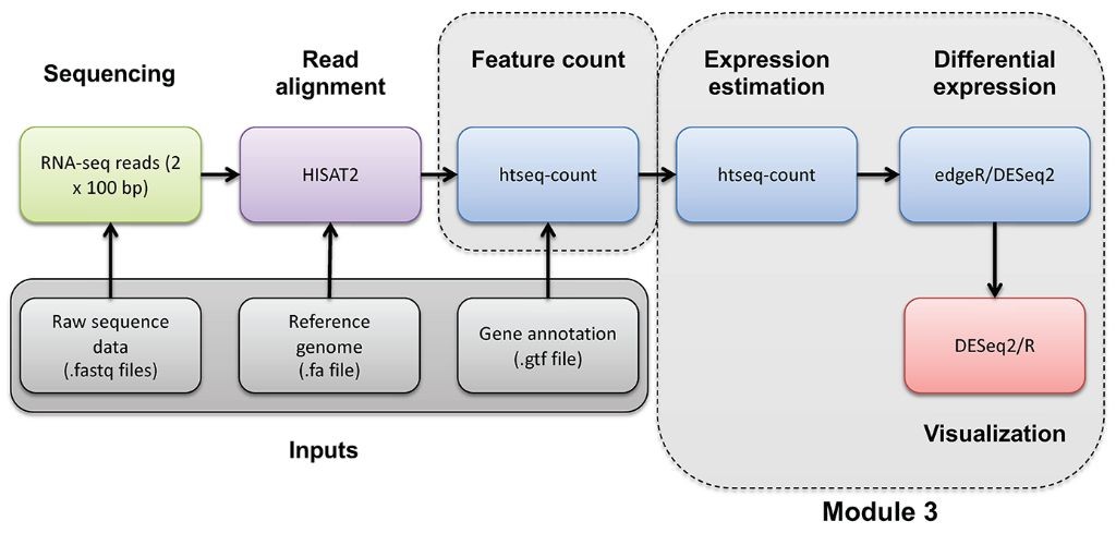
Bioconda recipe for RNA-seq analysis using HISAT2

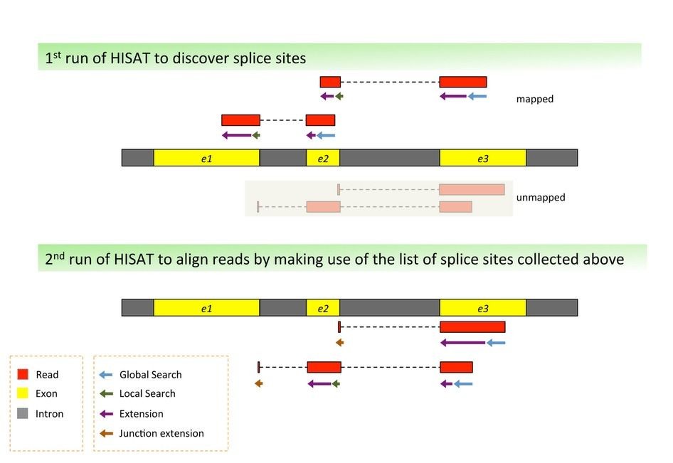
This recipe provides a streamlined process for performing RNA-seq analysis using HISAT2, a popular aligner for high-throughput sequencing data. The resulting alignment will serve as the foundation for downstream bioinformatics tools and pipelines.

Ingredients:

– Fastq files (RNA-seq reads)
– Reference genome in FASTA format
– HISAT2 executable
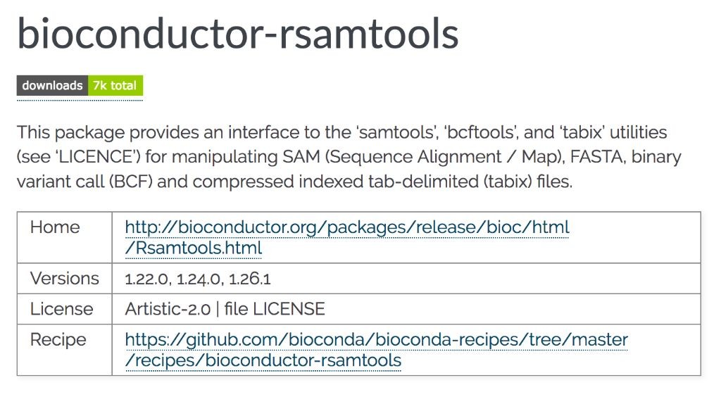
– SAMtools executable
– Optional: annotation file (e.g., GTF/GFF)

Step-by-Step Instructions:

1. Index the reference genome: Run `hisat2-build -p 4 reference.fasta indexed_reference`
2. Align RNA-seq reads: Run `hisat2 -p 8 -x indexed_reference -U read_1.fastq read_2.fastq > alignment.sam`
3. Sort and index SAM file: Run `samtools sort -@ 8 alignment.sam alignment_sorted.bam`
4. Convert to BAM and compress: Run `samtools view -bS alignment_sorted.bam > alignment.bam`
5. Optional: Add annotations: Run `gtf2samstdin < annotation_file.gtf > annotated_alignment.bam`

Cooking Time: ~30 minutes (depending on compute resources)

Bioconda recipe for variant calling with GATK

This recipe provides a straightforward guide to performing variant calling using GATK (Genomic Analysis Toolkit). With this recipe, you’ll be able to identify and annotate genetic variants from your genomic data.

Ingredients:
– GATK jar files (e.g., gatk.jar)
– BAM file containing aligned sequencing reads
– Reference genome in FASTA format
– Variant calling parameters (e.g., -min_alt_alleles 2)

Step-by-Step Instructions:

1. Download and install the GATK package if you haven’t already.
2. Run the following command to perform variant calling:

`java -jar gatk.jar HaplotypeCaller -I input.bam -R reference.fasta -o output.vcf -min_alt_alleles 2`

Replace `input.bam` with your BAM file, `reference.fasta` with your reference genome FASTA file, and `output.vcf` with the desired output VCF file.
3. Wait for the variant calling process to complete (this may take some time depending on the size of your data).

Cooking Time: The running time will depend on the size of your input BAM file and the computational resources available.

Bioconda recipe for metagenomics analysis using MetaPhlAn

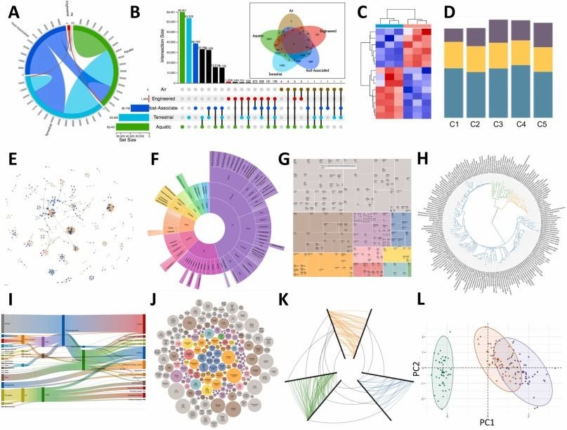
This recipe provides a step-by-step guide to performing metagenomics analysis using MetaPhlAn, a popular tool for profiling microbial communities from high-throughput sequencing data.

Ingredients:

– FASTA file of assembled contigs or reads
– MetaPhlAn database (downloaded separately)
– Bowtie2 alignment software
– Python and R programming languages

Instructions:

1. Install MetaPhlAn and its dependencies using Bioconda.
2. Preprocess your sequencing data by trimming adapters and filtering for quality using tools like Trimmomatic and FastqQC.
3. Align your preprocessed reads to the MetaPhlAn database using Bowtie2.
4. Run MetaPhlAn on your aligned reads, specifying the desired abundance cutoff and output format.
5. Use Python and R scripts (included with MetaPhlAn) to analyze and visualize your results.

Cooking Time: 1-2 hours

Bioconda recipe for ChIP-seq analysis with MACS2

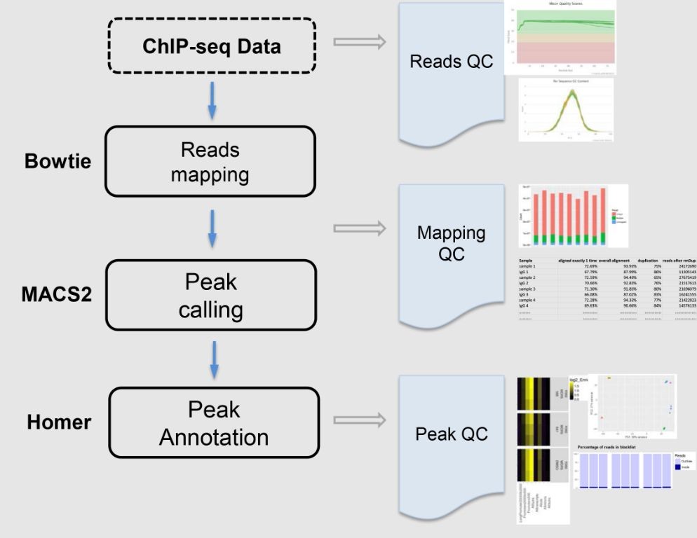
This recipe provides a step-by-step guide for performing ChIP-seq analysis using MACS2, a popular tool for identifying genomic binding sites from ChIP-seq data.

Ingredients:

– 1. Input BAM file containing ChIP-seq reads
– 2. Reference genome (FASTA or GTF format)
– 3. Peak calling parameters (e.g., p-value threshold, peak width)

Instructions:

1. Preprocess the input BAM file using tools like Picard (e.g., `picard MarkDuplicates`) to remove duplicates and trim adapter sequences.
2. Run MACS2 with the following command:
“`
macs2 callpeak -t -n -g -p 0.01 -w 200
“`
Replace `` with your input BAM file, `` with a desired prefix for the output files, and `` with the path to your reference genome.
3. Inspect the output peak file (.BED) and any additional visualization plots generated by MACS2.

Cooking Time: ~30 minutes (depending on computational resources and input data size)

Bioconda recipe for phylogenetic tree construction using RAxML

This recipe provides a straightforward guide to constructing a phylogenetic tree using RAxML (Randomized Axelerated Maximum Likelihood) and Bioconda. With this tool, you can analyze the evolutionary relationships between your favorite organisms.

Ingredients:

– A multiple sequence alignment file in FASTA format (e.g., your_genomes.fasta)
– A set of parameters for RAxML (see below)

Instructions:

1. Install RAxML and Bioconda using conda: `conda install -c bioconda raxml`
2. Load the multiple sequence alignment file into RAxML: `raxml -s your_genomes.fasta`
3. Specify the model parameters:
– `-p`: Set the number of bootstrap replicates (e.g., 100)
– `-f`: Choose the model type (e.g., GTR+G for nucleotides or PROTCATWAGL for proteins)
4. Run RAxML: `raxml -p 100 -f GTR+G -# your_genomes.fasta`
5. Parse the output to generate a Newick file: `raxml -o your_tree.nwk`

Cooking Time: ~30 minutes (depending on computational resources and alignment size)

This recipe should give you a good starting point for constructing a phylogenetic tree using RAxML and Bioconda. Happy analyzing!

Bioconda recipe for differential gene expression analysis with DESeq2

Perform differential gene expression analysis using DESeq2, a popular R package for identifying differentially expressed genes between biological conditions.

Ingredients:

– RNA-seq data (in FASTQ format)
– DESeq2 package
– R programming language
– Optional: additional packages for data visualization and annotation

Instructions:

1. Install DESeq2: Run `install.packages(“DESeq2”)` in your R console.
2. Load the data: Use `readRDS()` or `read.table()` to load your RNA-seq data into R.
3. Create a DGEList object: Use `DESeqDataSetFromMatrix()` to create a DESeq2 object from your count data and sample information.
4. Filter and normalize the data: Apply filtering and normalization using `DESeqStats()` and `rlogTransformation()`.
5. Perform differential expression analysis: Run `nbinomTest()` or `waldTest()` to identify differentially expressed genes between conditions.
6. Analyze results: Visualize and interpret your results using packages like `ggplot2` and `annotation`.

Cooking Time: Approximately 30 minutes, depending on data size and computational resources.

Bioconda recipe for protein sequence alignment using Clustal Omega

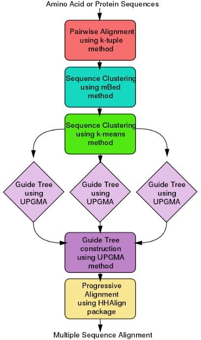
Align multiple protein sequences using Clustal Omega, a powerful tool for phylogenetic analysis. This recipe demonstrates how to align protein sequences and generate a visual representation of the results.

Ingredients:

– Protein sequence files in FASTA format (e.g., `sequence1.fasta`, `sequence2.fasta`)
– Clustal Omega software (part of Bioconda)
– A Linux-based environment (e.g., Docker container, local machine)

Instructions:

1. Install Clustal Omega using Bioconda: `conda install -c bioconda clustalo`
2. Create a new directory for your alignment project and navigate to it
3. Copy your protein sequence files into this directory
4. Run the following command: `clustalo -i -i … -o output.aln` (replace `` with your actual file names)
5. The alignment will be generated in the specified output file (`output.aln`)
6. Visualize the alignment using a tool like Jalview or SeaView

Cooking Time:

– Approximate time for installation and alignment: 15-30 minutes (dependent on computational resources)

Bioconda recipe for SNP annotation with SnpEff

A comprehensive annotation of single nucleotide polymorphisms (SNPs) is crucial for understanding their functional impact and predicting the effects on gene regulation. This recipe provides a step-by-step guide to annotating SNPs using SnpEff, a popular tool for predicting the consequences of sequence variations.

Ingredients:

– A VCF file containing the SNP data
– The SnpEff database (e.g., snpEFF_5.0gbd)
– A Unix-like system

Instructions:

1. Install SnpEff and its dependencies using Bioconda: `conda install -c bioconda snp-eff`
2. Load the SnpEff database: `snpEff -v -i vcf4.1 -d -o output.vcf input.vcf`
3. Annotate SNPs with SnpEff: `snpEff -v -i vcf4.1 -o output_ann.vcf output.vcf`

Cooking Time: ~5 minutes

This recipe provides a basic guide for annotating SNPs using SnpEff. For more advanced options and parameters, refer to the official SnpEff documentation.

Bioconda recipe for transcriptome assembly using Trinity

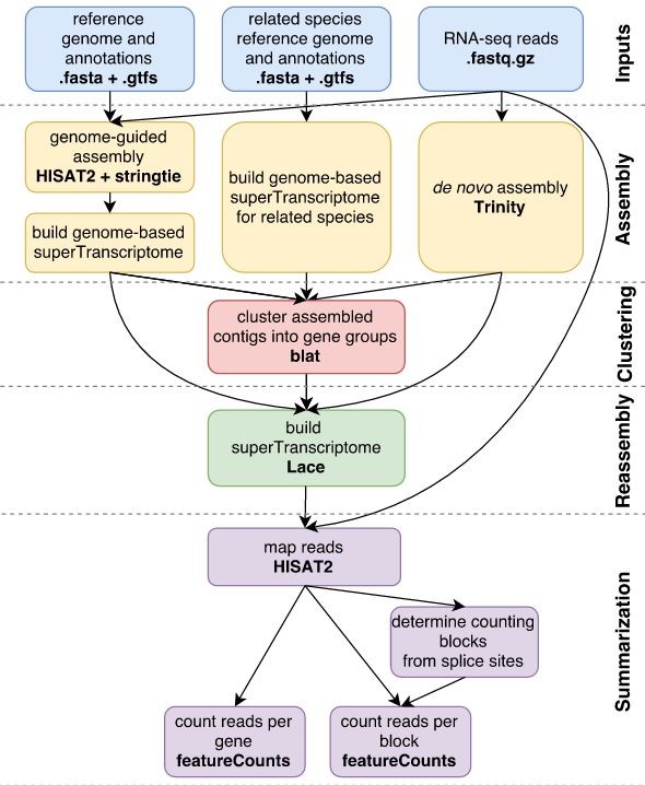
This recipe assembles transcriptomes from RNA-seq data using Trinity, a popular tool for de novo transcriptome assembly.

Ingredients:

– RNA-seq fastq files (e.g. paired-end or single-end)
– Trinity software
– Computing resources (CPU, memory, and disk space)

Instructions:

1. Prepare the input files: Ensure your RNA-seq data is in fastq format and stored in a directory.
2. Run Trinity: Use the following command:
“`
trinity –seqType fq –left –right –CPU
“`
Replace `` and `` with your actual file names, and `` with the number of CPU cores available on your machine.
3. Assemble the transcriptome: Trinity will generate a set of contigs (assembled transcripts) in a directory named `Trinity.fasta`.
4. Post-processing: Use tools like TransDecoder or AUGUSTUS to predict functional annotations for the assembled transcripts.

Cooking Time: approximately 2-10 hours depending on the size of your input data and computing resources.

Bioconda recipe for microbiome analysis with QIIME2

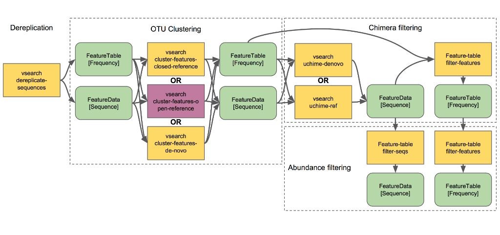
This recipe provides a straightforward guide to perform microbiome analysis using QIIME2. With this recipe, you’ll be able to demultiplex sequencing data, align reads to reference genomes, and generate taxonomic profiles for your samples.

Ingredients:

– QIIME2 installation (available from Bioconda)
– FASTQ files of sequencing data
– Reference genome(s) in FASTA format
– Sample information file (.tsv)

Step-by-Step Instructions:

1. Install QIIME2 using Bioconda: `bioconda install qiime2`
2. Demultiplex FASTQ files using `qiime tools demux`: `qiime tools demux –i-demultiplexed-seqs output/demultiplexed_seqs.qza –o-per-sample-sequences output/per_sample_sequences.qza`
3. Align reads to reference genomes using `qiime alignment align`: `qiime alignment align –i-demuxed-seqs output/per_sample_sequences.qza –i-reference-genomes input/reference_genome.fasta –o-aligned-reads output/aligned_reads.qza`
4. Generate taxonomic profiles using `qiime taxa classify`: `qiime taxa classify –i-aligned-reads output/aligned_reads.qza –i-taxonomy input/taxonomy.tsv –o-classified-table output/classified_table.qza`

Cooking Time: approximately 1 hour (depending on computational resources and dataset size)

Bioconda recipe for structural variant detection using Delly

This recipe provides a simple and efficient way to detect structural variants (SVs) from short-read sequencing data using Delly, a popular tool for SV detection. By following this recipe, you can identify various types of SVs, including insertions, deletions, duplications, inversions, and translocations.

Ingredients:

– Delly software
– Short-read sequencing data (FASTQ files)
– Reference genome sequence (FAI/FASTA file)

Step-by-Step Instructions:

1. Install Delly using Bioconda: `conda install -c bioconda delly`
2. Index the reference genome: `delly index -g .fa` (replace `` with your reference genome name)
3. Map reads to the reference genome: `delly map -o output.sam -p 4 -t 8 .fastq .fastq`
4. Detect structural variants: `delly call -g .fa -m output.sam -v output.vcf`

Cooking Time: approximately 30 minutes (dependent on computational resources and data size)

Bioconda recipe for gene ontology enrichment analysis with topGO

This recipe provides a step-by-step guide for performing gene ontology enrichment analysis using the topGO package in Bioconda. This analysis is useful for identifying biological processes and molecular functions that are overrepresented among a set of genes.

Ingredients:

– Gene expression data (e.g., GSE files) from a specific organism
– Functional annotation file (e.g., GOSlim format)
– topGO package installed in Bioconda

Instructions:

1. Load the gene expression data using `R` or `Python`.
2. Convert the functional annotation file to a suitable format for topGO.
3. Run `topGO` with the following command:
“`R
library(topGO)
go_terms <- GO_term(gene_expression_data, annotation_file, "BP") # Set 'BP' for biological processes enrichment_results <- go_enrichment(go_terms, p.value = 0.05) # Set your desired P-value threshold ``` 4. Visualize the enrichment results using a bar plot or heatmap. Cooking Time: Approximately 10-15 minutes

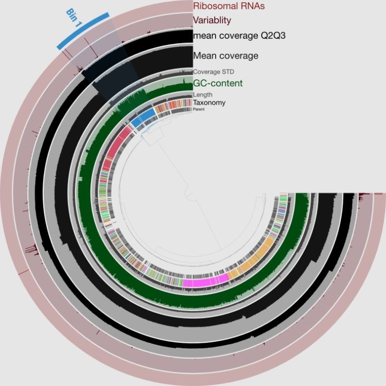
Bioconda recipe for genome annotation using Prokka

Prokka Genome Annotation Recipe

Prokka is a popular tool for rapid and efficient genome annotation. This recipe guides you through the process of annotating your genome using Prokka.

1. Ingredients:
   – Your genome sequence in FASTA format
   – A Prokka installation (available on Bioconda)
2. Step-by-Step Instructions:
   1. Install Prokka using Bioconda: `conda install -c bioconda prokka`
   2. Run Prokka on your genome sequence: `prokka –outdir output –genus your_genome.fasta`
   3. Customize the annotation by adding additional parameters (e.g., `–kingdom Archaea` or `–rRNA “)
3. Cooking Time: ~30 minutes to 1 hour, depending on the size of your genome and computational resources

Bioconda recipe for single-cell RNA-seq analysis with Seurat

This recipe provides a basic guide for conducting single-cell RNA-seq analysis using the Seurat package in Bioconda. By following these steps, you can efficiently analyze your single-cell RNA-seq data and visualize meaningful results.

Ingredients:

– bioconda/seurat (install via `bioconda install seurat`)
– Single-cell RNA-seq data in FASTA or FASTQ format
– R environment with Seurat package installed

Instructions:

1. Load the Seurat library: `library(Seurat)`
2. Load your single-cell RNA-seq data into R using `CreateSeuratObject()`
3. Perform quality control and filtering using `FilterCells()` and `FilterFeatures()`
4. Scale and normalize the data using `ScaleData()` and `NormalizeData()`
5. Perform dimensionality reduction using `PCA()` or `tsne()`
6. Visualize the results using `DimPlot()` or `FeaturePlot()`

Cooking Time: Approximately 30-60 minutes, depending on the size of your dataset

Bioconda recipe for sequence alignment using BWA

This recipe uses BWA (Burrows-Wheeler Aligner) to align high-throughput sequencing reads to a reference genome. The resulting alignment can be used for downstream analysis, such as variant detection and gene expression studies.

Ingredients:

– Reference genome in FASTA format
– Sequencing reads in FASTQ format
– BWA executable (available through Bioconda)
– Optional: additional parameters for advanced customization

Instructions:

1. Install BWA using Bioconda: `conda install -c bioconda bwa`
2. Download or create your reference genome and sequencing reads files.
3. Run BWA alignment: `bwa mem -x ont2d > aligned_sequences.sam`
4. Optional: customize alignment parameters using flags such as `-t` for thread count, `-R` for read group assignment, or `-Y` for advanced options.
5. Cooking time: approximately 1-10 minutes (depending on sequence length and computational resources)

Tips and Variations:

– Use `bwa mem -p` to output paired-end alignments
– Utilize `samtools` for downstream processing of the alignment file

Bioconda recipe for CRISPR guide RNA design with CRISPResso

Design efficient CRISPR guide RNAs using CRISPResso, a powerful tool for genome editing.

Ingredients:

– CRISPResso software
– Genome sequence (FASTA file)
– Target site information (e.g., gene name, position)

Step-by-Step Instructions:

1. Download and install CRISPResso.
2. Load the genome sequence FASTA file into CRISPResso.
3. Enter the target site information.
4. Run the “Guide RNA Design” module to identify potential guide RNAs.
5. Filter results based on desired criteria (e.g., specificity, efficiency).
6. Select the most suitable guide RNA(s) for your experiment.

Cooking Time:

– Preparation: 10 minutes
– Execution: 1-2 minutes per target site
– Total time: 30-60 minutes

Tips and Variations:

– Use CRISPResso’s built-in guides (e.g., sgRNAs, tracrRNA) or design custom guides.
– Optimize guide RNA design parameters for improved specificity and efficiency.

Bioconda recipe for pathway analysis using KEGG

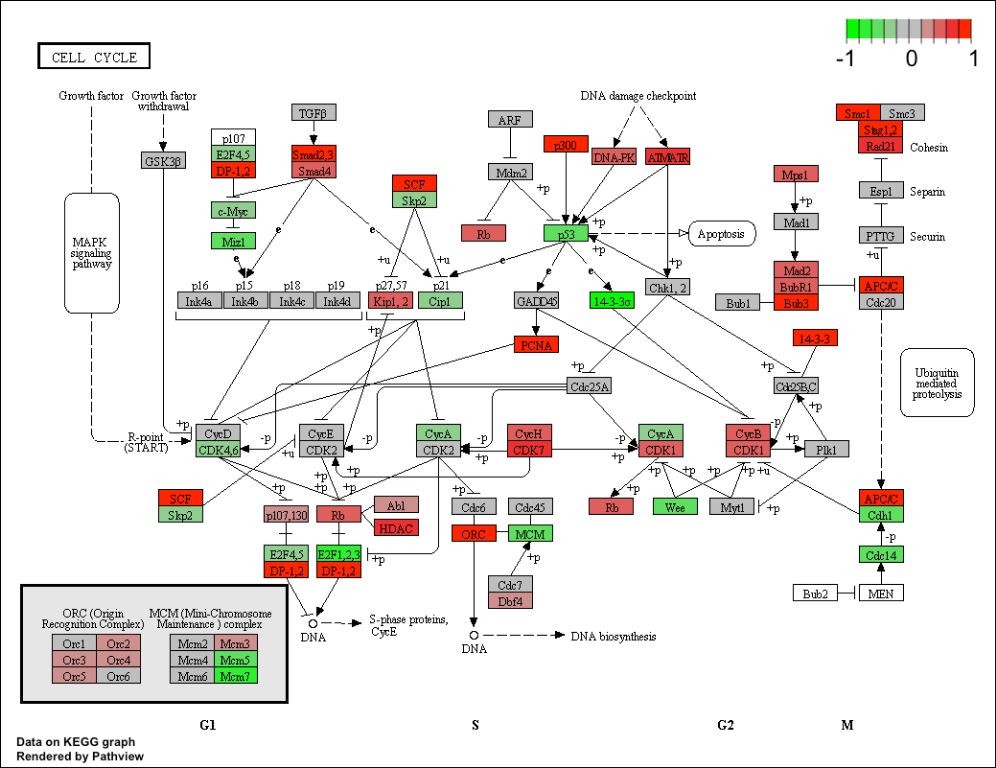
Quickly identify the key biological pathways involved in your dataset with this simple and efficient pipeline. This recipe uses Bioconda to install and configure tools for pathway analysis, leveraging the power of KEGG (Kyoto Encyclopedia of Genes and Genomes).

Ingredients:

– Conda environment
– bioconda
– kegg-annotate
– gsea

Steps:

1. Install the required packages by running `conda create -n kegg_pathway_analysis kegg-annotate gsea`
2. Activate the conda environment with `conda activate kegg_pathway_analysis`
3. Annotate your dataset using `kegg-annotate -i input_file -o output_file`
4. Run GSEA (Gene Set Enrichment Analysis) to identify pathways using `gsea -i input_file -o output_file`
5. Visualize the results with a tool like Cytoscape or Circos

Cooking Time: 10-15 minutes

Summary

Discover 18 essential Bioconda recipes for efficient bioinformatics workflows. These recipes cover a range of tasks, from genome assembly and variant calling to RNA-seq analysis and microbiome studies. Learn how to use tools like SPAdes, HISAT2, GATK, MetaPhlAn, MACS2, RAxML, DESeq2, Clustal Omega, SnpEff, Trinity, QIIME2, Delly, topGO, Prokka, Seurat, BWA, and CRISPResso. Each recipe provides a step-by-step guide to setting up and running the analysis, making it easy to get started with these powerful bioinformatics tools.